Working With R Files

Save your work to a .r file. Name yor file like _<.First Name>_HW4.
Upload your files to DropBox.

I have provided you with a .csv file called Insight.csv. It contains the log of my Honda Insight’s mileage since I bought it. There is a header row at the top of the spreadsheet. The columns are mostly self-explanatory, but just in case:

Date: the date of the fill up
Miles: the number of miles on the odometer when I filled up
Gallons: the number of gallons I put in the car
Price.per.Gallon: the price per gallon of gas
Total.cost: the total cost of the fillup (i.e., Price.Per.Gallon * Gallons)
Grade: the grade of gasoline purchased
MPG: the calculated miles per gallon for that tank (Miles/Gallons)
Price.Per.Mile: Total.cost/Miles
Cumulative.Miles: cumulative miles driven by the car
Cumulative.Gallons: cumulative gallons of gas purchased
Cumulative.Cost: cumulative cost of gas purchased
Cumulative.MPG: Cumulatove.Miles/Cumulative.Gallons
Cumulative.Price.per.Mile: Cumulative.Cost/Cumulative.Miles
Gas.Source: the chain of gas station the gas came from
Car.Said: the mileage for that tank that the car’s on-board computer reported
Delta: the difference between the mileage the car said and the mileage I calculated
Average.Price.of.Gas: cumulative average price paid per gallon of gas
Avg.Temp: average temperature for the period since the last fill-up, taken from a website at UD

Given this data, write an R script that will produce a SEPARATE WINDOW with this output.
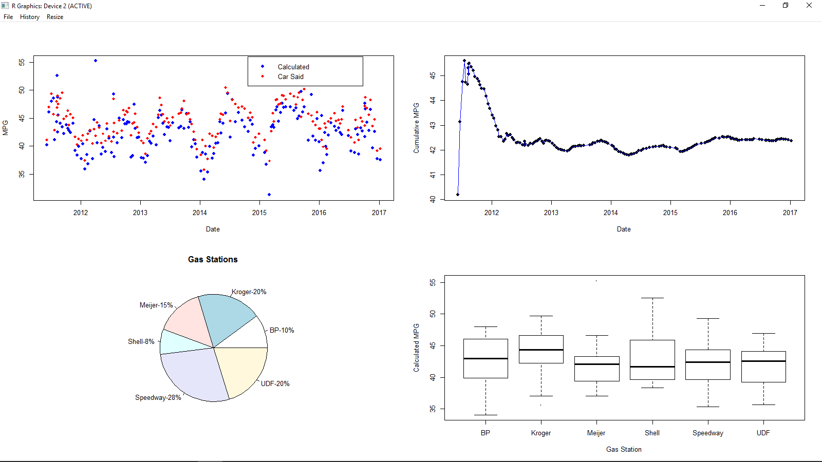
r statistics output.png

Note that the bottom right chart may not display all the labels on the X-axis until the window is maximized….that’s okay.

IMPORTANT NOTE: There are several gas stations that only have one or a small number of entries. Those should be INCLUDED in the data for the first two charts, but EXCLUDED when producing the bottom two charts. The following code will quickly accomplish this for you:

Assuming you have read the data into a dataframe called mileage:

tbl <- table(mileage$Gas.Source)
new.Mileage <- droplevels(mileage[mileage$Gas.Source %in% names(tbl)[tbl>10],,drop=FALSE])

The dataframe new.Mileage now has the data minus any entries where there were fewer than 10 observations at that Gas.Source.

Your script should begin with reading in the data. You can assume that your script and the data file are both in the working directory, so you need to only reference the filename (Insight.csv) and not worry about the file path.

  1. Write an R function called Cleaner that accepts a single vector of numbers that may contain NA entries and returns a vector where the NA’s have been replaced with -1.
  2. Write an R function that accepts three parameters: a lower bound, an upper bound, and an increment. Then use a repeat loop to generate a vector of the numbers from the lower bound to the upper bound by increment.
    For example, if my function was called counter
    answer <- counter(2,10,2)
    answer
    [1] 2 4 6 8 10
    i.e. the numbers from 2 to 10 in increments of 2
    answer <- counter(2,10,3)
    answer
    [1] 2 5 8
  3. Assuming I have three variables called lower, upper, and increment, how could I produce the same thing as number 2 with a single R statement that does not employ a loop?
  4. Write an R function that accepts two parameters: a vector of strings and a single search character. The function will then return a vector that contains the input strings that contain the search character.

For Example, if my function was called searcher
names <- c(“Bob”, “Bill”, “William”,”Tom”)
answer <- searcher(names,”i”)
answer
[1] “Bill” “William”

  1. Write an R function that accepts three parameters: a vector of strings, a single search character, and a single replacement character. The function will return the vector of strings, but with all instances of the search character replaced with the replacement character.
    For example, if my function was called replacer
    names <- c(“Bob”, “Bill”, “William”,”Tom”)
    answer <- replacer(names, “o”, “O”)
    answer
    [1] “BOb” “Bill” “William” “TOm"

    # Question 5

    byday <- table(FM$Date)

head(byday)

Average Number of Songs ListenedTo Over the Time Priod

avsongs <- mean(byday)
avsongs

Maximum Songs Listened To per Day

max(byday)

I have provided you with an Excel spreadsheet called Last_FM_data_shuffled.xlsx. It contains the log of all the music I have listened to on my phone since I began using the Last.fm website. As the name implies however, I have shuffled the entries so that they are no longer in chronological order. There is a header row at the top of the spreadsheet, and there are four columns of data: Band, Album, Song, and Date.

  1. Assuming you are not using packages that let you read from Excel, what must you do first in order to prepare this data to import to an R dataframe? What command will you use to import it?
    For this problem, submit a .r file where the first line is a comment telling me what you have to do, and the second line is the R command to import the data. Remember that # is the comment character.
  2. What is a single R command that can be used to count how many different bands are represented in the data file?
  3. Write an R script that will sort the data back into chronological order and store it in a new dataframe.
  4. Recall that the table() function can be used to quickly summarize data. As an example, assuming I have attached the dataframe with the song data, I can type

head(table(Song))

And get the following output

Song
(Song For My) Sugar Spun Sister 1901 45

                          2                        1               2

     50 Ways to Say Goodbye     6th Avenue Heartache      8:02:00 PM 
                          1                        2               1 

Each song title appears as a column heading and the number underneath it represents the number of time the song appears in the Song column of the dataframe.
Using this, what is the R command to determine the name of the song that has been played the most times? What is the R command to determine how many times that song has been played?

  1. Using R, determine the average number of songs I listened to per day over the time period in the dataset.

General Instructions

15 questions. The first 12 are fill-in-the-blank/short-answer type questions, while the final three require you to manipulate a dataset. You should have 4 Total files

For problems 13-15, assume that your script and the data file are both located in the current working directory. Therefore, when you read a file in, there is no need to provide a path, just the filename. For example:
myData <- read.csv(“inputFile.csv”, header=TRUE) CORRECT
myDaya <- read.csv(“C:\WSUDocs\Desktop\inputFile.csv”, header=TRUE) WRONG

When you are asked to write a function, all the information that function needs to operate should be included in the parameters. Thus, there should be no user input involved in the function itself.
For questions which ask you to produce a plot, you may use either base R plotting or ggplot2, whichever you prefer. Your plots should have appropriately labeled axes.

  1. Given a vector x:
    x <- c(4,6,5,7,10,9,4,15)

What R command could I use to find out how many entries in X are less than 7?

  1. Complete the following R command to generate a vector of the integers from 1:10

x <- 1______

  1. What is the default separator character in the paste() function?
  2. A categorical variable with a fixed number of levels is a _________________.
  3. _ changes the class of a variable, if possible.
  4. What function do you use in R to add a column to a matrix or data frame?
  5. Given the vector y:
    y <- c(101,85,97,102,76,89,95,94,90,80,82,75,103,100,79,69)

What R command could I use to replace any value greater than 100 with 100?

  1. Write a short R function called getNames that accepts two parameters called namesVector and excludeCharacter and returns all the entries in namesVector that DO NOT contain excludeCharacter.
  2. Would the following data be considered WIDE or LONG?
    Control Treatment Preheated Treatment Prechilled Treatment
    6.1 6.3 7.1
    5.9 6.2 8.2
    5.8 5.8 7.3
    5.4 6.3 6.9
  3. Given a matrix x, what R command would I type to return all the columns in row 5?
  4. Given two vectors:
    x <- c(3,2,4)
    y <- c(1,2)

The command z <- x*y will produce a vector z that contains (3,4,4). Explain why this happens.

  1. Write a short R function called replaceMean that accepts a parameter called numberData and returns a vector where any missing data has been replaced with the mean of data. For example
    x <- c(1.2, 7.9, 3.4, NA, 4.2, 9.1, NA)
    z <- replaceMean(x)
    z would now contain (1.2, 7.9, 3.4, 5.16, 4.2, 9.1, 5.16)
  2. I have provided you with a dataset in the file MetroMedian.csv. The file contains the median price per square foot of housing in each of the nation’s largest 557 metropolitan areas from April 1996 through December 2016. There are a number of missing entries where the data was not available.
    a. Read this file into a dataframe called metro
    b. This data is not correctly formatted. Produce a dataframe called tidyMetro that is suitable for analysis.
    c. For the entire data set, what is the mean value for the STATE of New York? Show both the R command(s) and the result
    d. Write an R function that accepts two parameters called valueFrame and searchRegion and returns the mean value for all entries for that region.
  3. I have provided you with a dataset in the file BeachWaterQualiy.csv. The file contains the bacterial count results from New York beaches from May 2005 to May 2016.
    a. Read this file into a dataframe called beaches
    b. When there was no detectable level of bacteria, the Results field was left blank. These fields were read into the dataframe as NA. Write a single line of R to replace any NA values in the Results column with 0 (zero).
    c. The sample dates recorded in this dataset are not suitable for ordering the data chronologically. Add a column to the beaches dataframe called new.date that is suitable for sorting.
    d. Write an R function called beachPlot that accepts three parameters called beachData, beachName, and sampleLocation. Your function should produce a line plot of the sample results for the named beach and sample location. For example, if I were to call
    beachPlot(beaches, “MANHATTAN BEACH”, “Center”)
    the function would return a plot that looked similar to

You may assume the dataframe being passed into the function has a column with a sortable date, but you cannot assume that the dataframe is chronologically sorted.

  1. I have provided you with a dataset in the file insight.csv. This is the mileage data (again) for my Honda Insight.
    a. Read this file into a dataframe called mileage
    b. Produce and label a scatterplot with blue points that puts Average Temperature on the x-axis and MPG on the y-axis
    c. Add a blue line that fits a linear model
    d. Add red points the put Average Temperature on the x-axis and the “car.said” mileage on the y-axis
    e. Add a red line that fits a linear model
    f. Add a legend that tells me which points are “Measured MPG” and which points are “Car Reported MPG”. You can specify the location of the legend or let the user select it, whichever you wish.

A datafile containing all the values has been attached here with;-
R.docx

Data Analytics using Regression Model

Suppose that a resource allocation decision is being faced whereby one must decide how many computer servers a service facility should purchase to optimize the firm’s costs of running the facility. The more servers they have, the less workers are needed. Too many servers will result in over-capacity and waste resources. The firm’s predictive analytics effort has shown a growth trend. A new facility is called for if costs can be minimized. The firm has a history of setting up large and small service facilities and has collected the 40 data points. Let’s consider the following linear model, and estimate that using the data.

Linear Model 2023-03-22T06:18:23.png

Where COST = the total cost to maintain a service facility.

         X  = the number of servers installed in each service facility

Using the Excel data, copy and paste to MINITAB answer the following questions.

1) Estimate the model and copy and paste the results and explain the meanings of the estimated coefficients.
2) Find TSS, RSS, ESS and R square, and carefully explain their meanings.
3) Using t test, prove/disprove if the estimated coefficient b is significant
4) What are the elasticity of server on total cost if you have 20 servers, or 40 servers?

5) Let’s consider the following log linear model
2023-03-22T06:19:46.png

Explain the coefficient of b and find the elasticity of number of server on the total cost.

6) Linear and Nonlinear Polynomial Models (1 point each)

2023-03-22T06:20:31.png
2023-03-22T06:20:49.png
2023-03-22T06:21:07.png

a. Estimate the model and copy and paste the results and perform the F test for each model
b. Let’s compare the two models, the Linear vs. Nonlinear models. In terms of goodness-to-fit, which one fits better? Carefully explain.
c. According to each model, what are the total cost to maintain the facility if you want install 10, 20, 50 servers?
d. Choose the best model from the regression model in terms of goodness-to-fit, and find the number of servers to minimize the total cost of the service facility.

II. Single Family House Sales in Chicago
We obtain a house sales data from the local Multiple Listing Service (MLS) who provides the up-to-date real estate market listing prices. We obtain the following variables from the properties listed in Chicago in 2015.
BEDROOM : Number of Bedroom
BATHROOM : Number of Bathroom
SQFT : Square Feet of Living Area
GARAGE : Number of Cars in Garage
AGEBLD : Age of Building
FIREPLACE : Number of Fireplace
ZIP : Zip Code
PRICE : Listing Price

  1. Find the descriptive statistics of Listing Price (PRICE) for two zip codes separately, and compare their central tendency, and variance using the following hypothesis tests: (1 points each)
  2. Simple Regression Model (Estimate separate model for each zip code)
    Let’s consider the following simple regression model:
    2023-03-22T06:22:21.png
    1) Estimate the simple regression model, and copy and paste the results from Minitab Regression output from Minitab and explain the meaning of coefficients from each model. (1 point)

2) Using the simple regression output find the following statistics. (0.5 point each)
) Estimate the simple regression model, and copy and paste the results from Minitab Regression output from Minitab and explain the meaning of coefficients from each model. (1 point)

2) Using the simple regression output find the following statistics. (0.5 point each)

Statistics ZIP CODE 1 = ZIP CODE2 =
a. Estimated intercept
b. Estimated slope coefficient
c. Total Sum of Square (TSS)
d. Regression Sum of Square (RSS)
e. Error Sum of Square (ESS)
f. R2
g. Adjusted R2
h. Variance and standard error of b1
i. Correlation Coefficient between listing price (PRICE) and square feet (SQFT)
j. Variance of et

  1. Nonlinear Model (Estimate separate model for each zip code, 1 point each)
    Let’s consider the following log transformed model.

1) Estimate the model and copy and paste the results, and explain the meanings of the estimated slope coefficients from each regression model.

2) Compare and explain the elasticity of square feet to price between two zip codes, which is

  1. Multiple Regression Model (Estimate separate model for each zip code, 1 points each)

1) Estimate the model using Minitab, and copy and paste the results.
2) Explain the meanings of the estimated coefficients.
3) Perform the t tests to find which variables are significant. List all significant variables at 5% and 10% significance levels.
4) Perform the F test for the each regression model, explain your verdict from the test.
5) Let’s compare the simple regression and the multiple regression models for each zip code. Carefully explain which is better.

6) Challenging model (3 points)
Now let’s find the best model to explain the listing price using the given variables. Any combination or any different functional forms are allowed. Find the best possible model. After deciding your final model, justify why your model is better than the other models.